Every logistics team working to optimize supply chain performance or reduce Scope 3 shipping emissions eventually runs into the same problem: the data available is not granular enough to act on.
Industry methodologies such as Clean Cargo assign emissions intensities at the trade-lane level, while carriers offer calculators based on aggregate historical data. Both approaches generate numbers. Neither generates operational intelligence, because neither reflects what actually happened on the voyage carrying your cargo.
This limitation becomes more critical as maritime disruption intensifies. UNCTAD highlights that disruptions in the Red Sea, Suez Canal, and Panama Canal are forcing vessels onto longer routes, increasing transit times and adding emissions pressure across global shipping networks.
This distinction matters more than it may seem. Two voyages departing from the same port, bound for the same destination, and operated by the same carrier can produce significantly different emissions intensities. Utilization, routing, port dwell time, and vessel speed vary across each voyage. Averages flatten these differences, obscuring the operational drivers of inefficiency.
Key takeaways:
- Shipment-level data reveals that emissions vary significantly between voyages, even on the same trade lane
- This analysis of 2025 voyages shows how operational factors such as routing, port time, utilization, and speed drive inefficiencies
- By examining high-intensity voyages, this article highlights where and why industry averages fail to capture optimization opportunities
In 2025, VesselBot tracked more than 5,800 containerships across global trade lanes. Among the voyages recorded, 3,899 fell into the high-intensity category, defined here as voyages recording a Well-to-Wake emissions intensity of at least 800 g CO₂e per TEU km. This analysis examines what those voyages reveal about the operational drivers of inefficiency, with a focused look at the port complex of Los Angeles and Long Beach.
What is Well-to-Wake intensity in Shipping Emissions?
Well-to-Wake (WTW) intensity measures the CO₂ equivalent emitted against the transport work generated by a voyage. It is expressed in grams of CO₂e per TEU kilometer.
A voyage that moves a large volume of cargo over a long distance produces significant transport work. Emissions are allocated across more unit-kilometers, lowering the measured intensity. A voyage that moves little cargo over a short distance generates proportionally less transport work, concentrating emissions and driving intensity upward.
WtW intensity, rather than total emissions, is therefore the correct lens for comparing voyage efficiency. It measures emissions relative to the actual work the vessel performs.
What Factors Affect Shipping Emissions in Ocean Freight?
There are multiple factors that affect the Well-to-Wake Intensity a vessel records in a voyage. The most important of them are as follows:
- Vessel Size & Utilization
- Routing
- Port Call Duration
- Speed
Vessel Size & Utilization
Larger vessels can carry more TEU, and, therefore, their emissions, even if significantly higher compared to smaller vessels, are allocated to more cargo. Of course, the benefits increase with utilization. A low-utilization voyage will be less efficient than one with higher utilization. A general rule of thumb is that the closer the TEU carried to the total capacity of the containership, the more efficient the voyage.
A VesselBot carrier benchmarking case study illustrates this point in practice. A shipper using the same carrier and similar shipment volumes still saw emissions rise. VesselBot found that switching to a better-performing service could reduce emissions intensity by 24%, from 93.9 to 71.7 g CO₂e per TEU km.
Routing
The route a vessel follows during a voyage gravely affects its Well-to-Wake intensity. Longer distances typically lead to greater efficiency because the vessel generates more transport work, even if its fuel consumption and emissions rise. The general principle is that out of all the different ways to travel from port A to port B, the most efficient one will be the one that is both:
- closest to the Minimum Feasible Distance required to reach port B after departing from port A, and
- including the fewest port calls
A Shanghai–Barcelona voyage case study shows how material this routing decision can be. VesselBot compared ocean freight options under Red Sea disruption conditions and found that the fastest ocean option was only 3% faster than the lowest-emissions option but produced 76% more emissions.
Port Call Duration
During port calls, vessels continue to burn fuel to maintain necessary operations. However, because the vessel is idle, no transport work is generated to offset emissions. Therefore, the general rule of thumb is that the less time a vessel spends in port, the better for its Well-to-Wake emissions intensity.
This is consistent with VesselBot’s Port Performance 2025 report, which found that vessels spent an average of 7 hours at anchorage and 18.7 hours at berth per port call in 2025, with port-call emissions averaging 25 tons CO₂e. The report also shows that port performance varies substantially by region, with average port call duration ranging from 19.8 hours in China/East Asia to 47.4 hours on the West Coast of North America.
Speed
Speed is a complex factor, as vessels are equipped with engines designed to operate optimally within specific thresholds. When the vessel's speed falls outside the optimal range, fuel consumption increases, as do emissions and Well-to-Wake emissions intensity.
Other factors
Apart from the main ones analyzed above, we should also consider other voyage-specific factors. For instance, if a vessel encounters extreme weather conditions, its fuel consumption will likely increase, reducing its efficiency. Another example would be voyages destined for congested ports; increased waiting times translate into higher fuel consumption without additional transport work. As already explained, this would lead to decreased efficiency.
What Inefficient Voyages Reveal about Shipping Emissions
In 2025, among the 5,816 container-carrying vessels VesselBot tracked, 1,379 collectively carried out 3,899 high-intensity voyages. The average Well-to-Wake emissions intensity of these voyages was 889.5 g CO2e per TEU km.
What stands out in those voyages is exactly what made them inefficient:
- Utilization was on average 38%, with vessels carrying an average of just 446 TEU
- The average distance covered was only 1,451 km.
- The time spent in port (2.35 days) almost reached the transit time needed to arrive at each port (2.45 days)
- The average speed was 13 knots
|
Voyages |
WtW Intensity (g CO2e/TEU km) |
Transit Time (days) |
Time in Port (days) |
Utilization |
TEU Carried |
Speed (knots) |
Distance (km) |
|
3,899 |
889.5 |
2.45 |
2.35 |
38% |
446 |
13 |
1,451 |
What was the destination of those voyages? One might expect that all those voyages were carried out across regional and backhaul routes. While this assumption generally holds true, it does not mean that these voyages departed from or arrived at only countries with lower demand and vessel traffic.
166 of those voyages included one or more US ports in 2025. Their average Well-to-Wake intensity was 892.8 g CO2e per TEU km, with vessels utilized at 29% capacity, carrying an average of 763 TEU and traveling 3,230 km at an average speed of 14.9 knots.
|
Voyages |
WtW Intensity (g CO2e/TEU km) |
Transit Time (days) |
Time in Port (days) |
Utilization |
TEU Carried |
Speed (knots) |
Distance (km) |
|
166 |
892.8 |
4.76 |
1.69 |
29% |
763 |
14.9 |
3,230 |
At the same time, that does not mean all those voyages were headed or departing from ports of low demand. In contrast, a few of them departed or headed to arguably the most vital port complex for containerized trade in North America, Los Angeles and Long Beach.
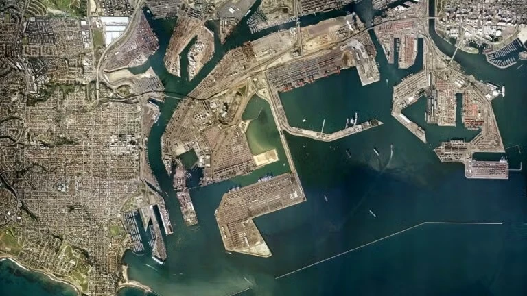
How the Los Angeles/Long Beach Complex Impacts Ocean Freight Emissions
In 2025, 16 voyages from or towards Los Angeles/Long Beach had an intensity of at least 800 g CO2e per TEU km. Does that mean voyages from or towards LA/LB are inefficient? Of course not. These voyages highlight just a fraction of the overall 1,577 containership voyages towards LA/LB in 2025, many of which fall into the most efficient intensity category.
Understanding what makes those 16 voyages stand out is vital to understanding what makes or breaks supply chain efficiency today.
Let’s focus on the port complex of Los Angeles and Long Beach, a key gateway for containerized trade in the United States. During 2025, 1,577 containership voyages departed or arrived at the port complex of LA/LB.
|
|
No |
WtW Intensity (g CO2e/TEU km) | Transit Time (days) | Time in Port (days) | Utilization | TEU Carried | Speed (knots) | Distance (km) |
|
High Intensity Voyages |
16 |
889.1 |
8.76 |
2.14 |
15% |
463 |
15.4 |
5,918 |
|
All Voyages |
1,577 |
127.7 |
11.94 |
2.74 |
74% |
6,204 |
16 |
8,810 |
|
Difference |
596% |
-27% |
-22% |
-80% |
-93% |
-4% |
-33% |
If we compare all voyages to the port complex with those of very high intensity, we observe significant differences across the board.
- Smaller vessel size and lower utilization: Ships were loaded 80% less, recording an average utilization of 15%, and carrying 93% fewer TEU (463 on average compared to 6,204).
- Shorter distances: The average distance on the most inefficient voyages towards LA/LB was 5,918 km, 33% shorter than the average of 8,810 km.
Overall, the above factors contributed to a 596% efficiency gap.
Many of those voyages are carried out by vessels moving cargo that has arrived in Los Angeles/Long Beach to other West Coast ports, mainly Oakland.
This is another instance that highlights the importance of supply chain visibility. A shipper sending cargo from Ningbo to Oakland would probably center their strategy around the important leg of the voyage (connecting China/East Asia to the West Coast of North America).
However, if you lack information about how many port calls the vessel made before delivering your shipment, whether your shipment was transshipped during a port call, or what the actual and operational profile of the vessel(s) carrying your shipment was, supply chain visibility is unattainable.
Conclusion
The analysis of 2025 voyages shows that inefficiency in ocean shipping is not driven by a single factor. Instead, it is the outcome of how vessel size, utilization, routing, port time, and operational speed interact during each individual voyage. Shipment-grade execution data reveals that the most polluting voyages are typically characterized by low utilization, shorter sailing distances, and operational patterns that generate emissions without proportional transport work.
The Los Angeles/Long Beach case illustrates this clearly. While the vast majority of voyages to the region operate efficiently, a small subset records Well-to-Wake emissions intensities, nearly up to six times higher than average. These voyages often involve lightly loaded vessels traveling shorter distances and serving redistribution routes along the West Coast, where cargo is repositioned after arriving at the main gateway ports.
For shippers’ logistics teams, the implication is straightforward: averages cannot capture these operational realities. Optimization strategies, decarbonization efforts, and cost-reduction initiatives must rely on shipment-level insights and execution data to identify where inefficiencies truly occur.
Without that level of insight, emissions remain a reporting metric. With execution-grade data, they become an operational variable that can be measured, managed, and reduced.
SOURCES:
About the author

Manos Charitos is Data Analyst at VesselBot, where he works with AIS-tracked voyage data, digital twin models, and shipment-level execution records to measure and interpret maritime emissions across global supply chains. The analysis in this article is his own work, drawn from 2025 voyage data across all major carriers. His background combines Mathematics and Shipping, giving him both the quantitative foundation to model emissions at the voyage level and the operational context to understand what those numbers mean for shippers making carrier and routing decisions.